Automated vs. Manual Port Cranes: Comparing TCO Under Different Utilization Rates

A terminal with uneven vessel arrivals can buy an automated crane system that performs well technically yet remains expensive per container move. Another terminal may keep manually operated cranes running across multiple shifts and find that staffing, shift coverage, and inconsistent output cost more than the automation premium. Automation generally makes the stronger financial case when sustained, achievable throughput spreads its additional fixed costs over enough moves and produces realizable operating savings. Manual operation can remain preferable when demand is low, volatile, or constrained elsewhere in the terminal.

The decision therefore depends on more than a quoted purchase price or maximum moves per hour. An evaluation of the total cost of ownership of automated port crane systems must connect utilization to staffing, integration, maintenance, and service continuity. A forecast that assumes full labor savings from commissioning, or treats crane capacity as guaranteed terminal throughput, can make the wrong option appear cheaper.

Start with an equivalent operating scope

“Automated” and “manual” are not sufficiently precise procurement categories. A manually operated crane may already include positioning assistance, anti-sway control, and equipment monitoring. An automated installation may still require remote operators for exceptions, supervision, or particular handling tasks. Remote operation alone does not mean the crane completes its working cycle autonomously.

Compare equipment performing the same duty: ship-to-shore cranes against comparable ship-to-shore cranes, or yard cranes against equivalent yard cranes. Differences in lifting capacity, stacking geometry, travel distance, and container mix can otherwise dominate the result. For a retrofit, assess the remaining mechanical life before committing to controls and software with a separate renewal cycle.

Define the system boundary before requesting commercial offers. Automation may require communications infrastructure, positioning systems, safety controls, terminal operating system interfaces, and changes to traffic management. Some costs serve a whole block or terminal rather than one crane. Allocate them consistently across alternatives; do not compare a complete automated installation with a manual crane purchase that excludes its supporting infrastructure.

Utilization needs a denominator—and a demand constraint

A crane can be scheduled for long hours but spend much of that time waiting for trucks, yard access, or vessel work. Conversely, short operating windows can involve intensive productive work. Using “hours switched on” as utilization conceals this distinction.

For commercial modeling, use a clearly stated measure such as:

Productive utilization = productive handling hours ÷ scheduled service hours.

Then reconcile those hours with completed moves using a sustainable handling rate. Record waiting, planned maintenance, equipment faults, weather interruptions, and operational restrictions separately. Availability measures whether equipment is ready to work; utilization measures how much it is used. Combining them without explanation makes both downtime costs and capacity assumptions difficult to audit.

Annual averages also hide the operating pattern. Concentrated vessel calls may require a large manual staffing roster even when annual utilization is modest. An automated system may reduce that coverage burden, but only if its supervision and exception-handling arrangements genuinely need fewer people. Examine shift-level demand alongside the annual total.

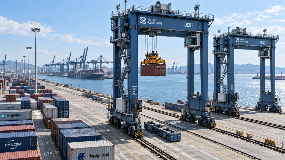
These are operating scenarios, not universal percentage bands. A utilization threshold from another terminal is not transferable unless the crane scope, cost structure, labor arrangements, and demand profile are comparable.

Build the cost model around costs that actually change

Capital and commissioning

Include equipment, installation, civil works attributable to the option, power supply, controls, communications, integration, testing, training, and commissioning support. Brownfield conversion may also require temporary operating arrangements while blocks or cranes are unavailable. These transition costs can materially alter the comparison with continuing manual operation.

Separate initial investment from later replacement obligations. Mechanical structures, drives, control hardware, servers, and software support may have different service lives. Use a common evaluation horizon and consistent residual-value assumptions. A lower purchase price does not necessarily imply a lower discounted ownership cost.

Staffing and support

Model staffed positions by shift, including relief coverage, supervisors, remote operators, exception handlers, maintenance technicians, and systems support. Do not convert every removed cab position directly into a cash saving. Labor savings become financial savings only when payroll, overtime, contractor expenditure, or future hiring actually falls.

Where employees are redeployed, show the avoided cost or additional productive work separately. Training and parallel operation during ramp-up belong in the transition budget. The steady-state staffing plan should also survive breaks, absence, peak exceptions, and recovery operations—not merely routine cycles.

Energy, maintenance, and digital obligations

Compare energy on both an annual and per-move basis, including idle consumption and relevant demand charges. Automated motion control may improve consistency, but energy outcomes also depend on drives, travel distances, load profiles, regeneration, and dispatching. Do not attribute savings from electrification or newer hardware entirely to automation.

Maintenance still includes mechanical inspections, wear parts, lubrication, and planned servicing. Automation adds sensors, networks, positioning equipment, software maintenance, cybersecurity work, and potentially specialized diagnostics. Request commercial terms for licenses, support renewals, upgrades, spare parts, and component obsolescence. Check which faults terminal staff can resolve and which require vendor intervention.

Calculate break-even without pretending throughput is guaranteed

Use discounted cash flow for the investment decision. For each option, calculate initial expenditure plus the present value of annual operating costs, replacement expenditure, and attributable disruption costs, less the present value of residual value. Apply the same currency basis, evaluation horizon, and discount-rate methodology to both alternatives. Keep inflation and nominal or real discount rates consistent.

A simpler annualized model helps explain the utilization effect:

Annual cost = annualized fixed cost + annual moves × variable cost per move.

When automation has higher fixed costs but lower variable costs, the indicative crossing point is:

Break-even annual moves = additional annualized fixed cost ÷ variable saving per move.

The numerator must include the net fixed-cost difference, not just the purchase-price premium. The denominator must reflect savings that can actually be captured. If automation does not reduce variable cost, there is no volume-based crossing point in this simplified model; the case must rest on other measurable benefits.

Real terminal costs are often stepped rather than linear. Opening another shift, adding a remote operator, or expanding maintenance coverage changes costs abruptly. Calculate separate operating bands where staffing or support changes instead of forcing one straight line through the entire demand range.

Convert the break-even volume into productive hours using the achievable handling rate. Then test whether that workload fits the operating calendar after maintenance and expected interruptions. If the threshold requires more work than the terminal can physically deliver, the apparent financial break-even is not an actionable investment case.

Different utilization patterns point to different choices

Low demand: protect against stranded fixed costs

When cranes spend substantial periods awaiting work, manual operation often benefits from lower initial complexity and less digital infrastructure to maintain. Its advantage is strongest where staffing can be adjusted economically. It weakens where minimum shift coverage, scarce operators, or irregular peaks create significant fixed labor costs.

Evaluate whether targeted assistance or remote operation addresses the actual bottleneck without purchasing full automation. Such alternatives still need their own cost and safety assessment, but they can separate an operator-location problem from a throughput problem. Forecast growth should not be treated as committed demand merely because automation creates available capacity.

Variable demand: test the shape of the workload

Two terminals with similar annual moves may have different economics if one operates steadily and the other experiences concentrated peaks. Manual staffing flexibility, overtime, automated supervision ratios, and exception frequency can change the preferred option.

Run scenarios for weaker demand, expected demand, and sustained growth, using supportable assumptions. Include a delayed ramp-up rather than assuming the eventual workload begins immediately. Where staged deployment is practical, account for duplicated interfaces and temporary mixed-operation costs; phasing reduces exposure only when those costs do not erase its flexibility.

High demand: verify system capacity and recovery

Sustained utilization gives recurring savings more opportunity to offset the investment premium. However, high demand also increases the cost of interruptions. Automated cranes cannot deliver extra terminal throughput if horizontal transport, stacking capacity, gate operations, or berth planning remain limiting factors.

Use acceptance criteria tied to the intended workflow, including exception handling and restart after faults. A nominal cycle rate achieved under favorable conditions is not equivalent to sustained output across normal container variation and traffic conflicts. Compare complete operating systems, not isolated machine speeds.

Downtime can reverse an apparently favorable result

Assess both routine equipment faults and shared-system failures. A fault in one manually operated crane may remain localized, although manual installations also depend on shared power and systems. Automation can introduce common dependencies through networks, servers, positioning infrastructure, or central control. Redundancy and segmentation can reduce that exposure, but their costs belong in the model.

Price disruption through identifiable consequences: overtime, temporary equipment, backlog recovery, contractual exposure where applicable, and displaced work. Avoid multiplying every lost hour by theoretical maximum revenue. Some moves are delayed rather than lost, and some disruption costs may overlap.

Fallback operation deserves specific scrutiny. Confirm whether degraded or manual modes exist, what equipment remains available, who is authorized and trained to operate them, and how long recovery takes. A fallback function has limited commercial value if the required personnel are unavailable or if restarting depends on specialist support outside the service window.

Turn the comparison into procurement conditions

Before approving the investment, translate the assumptions driving the preferred option into evidence requests:

• Throughput: require achievable operating rates under the specified layout, workload, and exception conditions.
• Staffing: document coverage by shift, supervision limits, and the actions needed to realize cash savings.
• Lifecycle support: obtain renewal terms, upgrade responsibilities, spare-part arrangements, and support response commitments.
• Integration: assign responsibility for interfaces, testing, data access, and changes to connected systems.
• Recovery: define fault scenarios, degraded operation, and acceptance tests for restoring service.

Prefer automation when its discounted cost advantage survives conservative demand, a realistic transition period, and credible disruption assumptions. Prefer manual operation—or a narrower automation scope—when savings depend on uncommitted growth, unchanged payroll being counted as avoided cost, or throughput unsupported by the rest of the terminal. A close result should trigger negotiation around the variables that could change the decision, rather than approval based on the most optimistic utilization forecast.