Bulk Materials Transport Pricing Drivers: How to Forecast Delivered Cost

A delivered-cost forecast for bulk material starts with a simple equation, but reliable approval depends on exposing the assumptions inside it:

Delivered cost per tonne = material purchase price + origin handling + line-haul transport + transfer and storage + destination handling + losses, claims, and contract contingencies.

Quoted freight is only one line in that equation. A low rail, truck, barge, or vessel rate can be offset by poor loading productivity, demurrage exposure, empty repositioning, excessive inventory at the destination, or a contract structure that transfers operational volatility into the delivered price. The forecast should therefore describe the physical movement of the material as clearly as it describes the commercial rate.

Start with the physical flow, not the carrier quote

Bulk logistics costs are shaped by the route's slowest and least reliable point. For aggregates, ore, coal, grain, cement clinker, fertilizers, and similar commodities, the relevant unit is often a tonne moved through a chain of equipment: mine or plant stockpile, feeder, conveyor, loader, rail wagon or truck, discharge system, terminal stockyard, and final receiving point. A rate that assumes uninterrupted flow becomes misleading when any part of that chain has limited capacity.

Map each handoff before building the budget. Record where title transfers, where material is weighed, where quality is sampled, where it is stored, and where responsibility for spillage, moisture gain, contamination, or shrinkage changes. These operational details determine whether a cost belongs in transport, handling, inventory, or a separate allowance. They also expose duplicated charges that are easy to miss when quotations are grouped under broad labels such as “terminal service” or “delivered freight.”

Haul distance matters, but distance alone is not a pricing driver. A longer unit-train route with high payload utilization and direct unloading can carry a lower cost per tonne than a shorter route requiring repeated truck movements and manual transfer. Likewise, a short port-to-plant leg can become expensive when gate access, berth windows, or receiving hours force equipment and crews to wait.

Separate fixed route cost from volume-sensitive cost

A defensible forecast distinguishes charges that change with tonnes from charges that continue even when throughput falls. This distinction is especially important when annual demand is uncertain or delivery is seasonal.

Fixed commitments should be converted into a cost per forecast tonne only after testing realistic utilization. Dividing annual equipment hire by maximum theoretical capacity creates an artificially low unit cost. Use the volume that can actually be loaded, moved, discharged, and received within the operating calendar. Planned maintenance, weather interruptions, destination shutdowns, and loading restrictions often reduce usable capacity well below nameplate capability.

A useful internal view presents three volume cases: committed minimum volume, expected operating volume, and high-throughput volume. The purpose is not to predict every variation. It is to show where the unit cost becomes sensitive to underutilized assets or contractual take-or-pay obligations.

Fuel exposure must match the transport mechanism

Fuel surcharges are commonly treated as a generic escalation line, yet their relevance differs materially by mode and contract. Trucking exposure is influenced by road distance, congestion, backhaul availability, axle limits, and idling at loading or receiving sites. Rail exposure is affected by locomotive efficiency, train length, grade, dwell time, and whether the operator applies a published surcharge formula. Marine legs may incorporate bunker adjustments, port waiting, and charter terms that distribute consumption risk differently.

Do not assume that an indexed fuel clause fully reflects fuel risk. Review the reference index, lag period, floor or cap provisions, currency basis, and whether the surcharge is applied to all invoice components or only base line-haul. A surcharge calculated on a rate that already includes a fuel allowance can create double recovery. Conversely, a fixed freight rate may conceal a short validity period followed by a broad repricing right.

Electric rail transport creates a different question. The commercial exposure may sit in traction-energy charges, access tariffs, or a carrier's generalized adjustment mechanism rather than a visible diesel surcharge. The forecast needs to identify the actual settlement rule, not merely label the movement “rail.”

Handling capacity often determines the true delivered rate

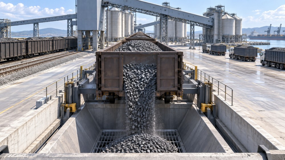
Bulk material handling is where nominal transport economics frequently break down. A train, truck fleet, or vessel earns its return while moving, but it accumulates cost while waiting to load or discharge. If a receiving hopper cannot accept the intended flow rate, each inbound unit stays in the cycle longer. More equipment is then required to deliver the same monthly tonnage, or deliveries slip and inventory must rise.

Examine loading and discharge as a cycle rather than isolated hourly capacities. The relevant question is not whether a conveyor is rated for a specified throughput; it is whether material can move at that rate through feeders, transfer chutes, screens, weighbridges, dust controls, stacker-reclaimers, and the receiving process without interruption. Wet, sticky, abrasive, oversized, or variable-density material can reduce effective throughput even when mechanical equipment appears adequate on paper.

Material properties also affect cleanup and loss assumptions. Fine powder may need enclosed transfer and dust collection. High-moisture material can bridge in hoppers, freeze in cold conditions, or add non-saleable water weight. Abrasive ore can increase wear at chutes and liners, creating maintenance windows that constrain dispatch. These effects should not be buried in an undifferentiated contingency; they belong in throughput, maintenance, handling, and loss assumptions where they can be challenged and updated.

Cycle time is a capital and operating-cost variable

For dedicated railcars or specialized trucks, calculate the complete turnaround cycle: loading queue, loading time, line-haul, terminal queue, discharge, inspection or cleaning, empty return, and any required repositioning. Equipment availability is driven by this full cycle. Reducing discharge dwell by a few hours may defer the need for additional rolling stock, while a recurring blockage at the destination may require extra units even if the haul distance remains unchanged.

The same logic applies to port movements. Berth productivity and yard congestion influence how long cargo remains tied to terminal capacity. A lower ocean or coastal freight quotation can lose its advantage when the receiving terminal lacks reclaim capacity or discharge windows. The forecast should model waiting as a costed condition, not as a footnote under “operational risk.”

Use contract terms to locate risk, not just compare headline prices

Two offers with similar delivered rates may place very different obligations on the purchasing side. The comparison should normalize scope before selecting the lower figure. Include loading, weighing, sampling, permits where applicable, access fees, equipment cleaning, detention, storage, rehandling, quality claims administration, and emergency transport requirements. A carrier's exclusion list can be more economically meaningful than its base rate.

Pay particular attention to four contract mechanics:

• Volume commitment: Minimum annual tonnage, monthly nominations, and take-or-pay provisions determine whether unused capacity remains payable during demand changes or plant outages.
• Service measurement: A rate is hard to enforce if the contract does not define the start and end of loading, free time at destination, acceptable queue conditions, and the records used to resolve disputes.
• Escalation and pass-through: Indexation should identify the index, calculation date, currency conversion method, and treatment of new route charges. Broad “cost increase” language prevents a stable budget.
• Performance relief: Force majeure, maintenance shutdowns, congestion, weather, and third-party infrastructure failures should be assessed against the party bearing standby, substitute transport, and inventory costs.

Contract risk has a timing dimension. A charge that is technically recoverable after a dispute may still create a cash requirement during the period in which invoices are paid. Forecasting should distinguish expected economic cost from temporary working-capital exposure when claims, weight differences, or service credits are settled later.

Build the forecast around assumptions that can be audited

A practical model does not need excessive precision. It needs traceable inputs, consistent units, and a clear link between operational assumptions and cost outputs. Keep tonnes, wet tonnes, dry tonnes, vehicle payload, train length, loading rate, dwell hours, storage days, and currency separate until the final calculation. Unit conversion errors are common when a purchase price is quoted on dry basis while transport and terminal charges are invoiced on received weight.

For each route segment, retain the source of the rate, validity period, included services, indexation method, assumed volume, and the operational condition required to achieve it. For example, a rail rate may presume block loading, a minimum consist size, a specified turnaround time, and a defined origin-destination pair. If the operating plan changes to partial loads, intermittent dispatch, or an alternative terminal, the original rate should not automatically carry forward.

Then stress the variables with the greatest economic leverage rather than applying a blanket uplift to every line. The right stress test often combines conditions that occur together: lower throughput lengthens cycle time; longer cycle time reduces asset availability; reduced availability raises hire or spot-market reliance; delayed deliveries increase terminal dwell or site inventory. Treating these as independent percentage changes understates their interaction.

Distinguish price volatility from design weakness

Some cost movements are external and visible, such as fuel indices, exchange rates, or published access tariffs. Others indicate that the logistics design is fragile. Repeated detention, variable payloads, missed loading windows, and frequent rehandling are not merely volatile expenses; they signal a mismatch between equipment, material characteristics, and operating schedule.

This distinction changes the response. Index-linked exposure can be managed through contractual formulas, scenario ranges, or timing of commitments. A design weakness requires operational correction: larger surge storage, different loading equipment, revised train or truck scheduling, improved discharge reliability, or a route with fewer constrained transfers. Adding contingency without identifying the cause preserves the same failure point in the approved plan.

Delivered-cost forecasting is strongest when the model remains tied to physical evidence: payload records, cycle-time observations, terminal invoices, equipment maintenance windows, and actual loss measurements. Each update should explain whether a variance came from market pricing, volume utilization, asset delay, handling performance, or a scope gap. That discipline turns a transport quote into a usable view of total logistics economics.