Bulk Material Transport: Comparing Truck and Overland Conveyor Costs

Which Option Is More Likely to Reduce Your Transport Costs?

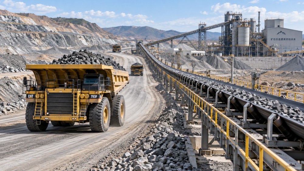
An overland conveyor deserves serious evaluation when substantial volumes move repeatedly between fixed locations. Its economic strength comes from spreading infrastructure costs across dependable production.

Trucks usually have stronger economics when destinations change, production remains uncertain, or the operation needs transport capacity quickly without committing to a permanent corridor.

Distance alone cannot settle the decision. A shorter, heavily utilized conveyor may outperform trucking, while a longer conveyor with intermittent demand may struggle financially.

The first management question is therefore straightforward: how much material will actually move over this route, for how many years, and with what certainty?

Compare the Complete Transport System Before Comparing Prices

A credible comparison starts with identical boundaries. Both alternatives must deliver the same material volume, between the same locations, at the same required service level.

Include loading, transport, unloading, and any intermediate storage or transfer equipment. Otherwise, a cheaper transport quote may simply exclude functions included in the competing proposal.

For trucking, capital expenditure includes vehicles, haul roads, drainage, workshops, fueling facilities, and traffic controls. Leasing or outsourcing changes payment timing but preserves underlying costs.

For conveyors, include civil foundations, structures, belts, drives, electrical distribution, transfer stations, controls, installation, and commissioning. Corridor access and permitting can materially affect the budget.

Existing infrastructure changes the result considerably. A serviceable road and available fleet can favor trucking, whereas expensive road construction may strengthen the conveyor business case.

Account for construction timing as well. Delayed commissioning can postpone production revenue, potentially outweighing several years of projected operating savings from a new conveyor.

Use supplier estimates with consistent scope, currency, escalation assumptions, and contingency allowances. Separate preliminary budget figures from engineered quotations before presenting an investment recommendation.

Where Do Operating Costs Actually Diverge?

Truck operating costs typically combine fuel, drivers, tires, maintenance, road upkeep, supervision, and fleet support. Their relative importance depends on local operating conditions and contracts.

Fuel consumption responds to payload, gradients, rolling resistance, queuing, and empty returns. A fleet’s nominal payload provides little insight without a realistic cycle-time model.

Conveyor operating costs include electricity, belt and idler replacement, maintenance labor, inspections, cleaning, and transfer-point upkeep. Lower staffing requirements do not eliminate maintenance responsibilities.

Conveyor energy demand depends on route length, vertical lift, belt resistance, loading, and drive efficiency. Request modeled consumption across expected operating loads, including partial utilization.

For both systems, calculate energy per delivered tonne using site-specific assumptions. Generic fuel or electricity benchmarks can mislead when terrain and utilization differ substantially.

Truck fleets offer incremental capacity adjustments, but additional shifts or vehicles can increase supervision and support costs. Conveyor expansion may require major drive or belt upgrades.

Automation can change the comparison. Autonomous trucks may reduce some staffing requirements, while introducing additional communications, integration, specialist support, and infrastructure costs into the model.

A Worked Cost Comparison: When Does the Conveyor Pay Back?

The following example demonstrates the calculation method using hypothetical inputs. These figures are illustrative assumptions, not supplier quotations, industry averages, or a forecast for any site.

Assume both systems can deliver three million tonnes annually over the same corridor for ten years. Apply an eight percent real discount rate throughout.

For simplicity, assume constant real costs, no residual value, and no interim capital replacements. Actual investment models should include replacement schedules, taxes, and working capital.

The capital recovery factor at eight percent over ten years is approximately 0.149. Multiplying initial investment by this factor converts capital into an equivalent annual cost.

Annualized truck capital costs approximately $0.745 million, while conveyor capital costs approximately $2.683 million. Adding operating expenditure produces a consistent annual comparison for both alternatives.

At three million tonnes annually, trucking costs approximately $2.45 per tonne. The conveyor costs approximately $1.79 per tonne, including annualized capital under these assumptions.

The conveyor therefore saves approximately $1.96 million in equivalent annual cost. This advantage depends on achieving the assumed volume and maintaining the modeled operating costs.

Its additional upfront investment is $13 million, offset by $3.9 million in annual operating savings. Simple incremental payback is approximately 3.3 years, before discounting.

At the stated discount rate, the present value of those operating savings is approximately $26.2 million. Subtracting additional investment yields about $13.2 million in incremental value.

Payback helps communicate funding exposure, but discounted cash flow should guide approval. It captures project duration and the timing of savings more accurately than payback alone.

Find the Throughput Threshold That Changes the Decision

The most useful output is often a break-even throughput estimate. It reveals how far production can fall before the preferred transport option loses its advantage.

Using the example, trucking has approximately $1.945 million in annual fixed and annualized capital costs. The conveyor’s corresponding total is approximately $3.583 million annually.

Dividing that $1.638 million difference by the $1.20 variable-cost saving gives a break-even volume of approximately 1.37 million tonnes per year under the illustrative assumptions.

Below that volume, trucking becomes cheaper in this simplified model. Above it, the conveyor benefits from spreading its higher capital commitment across more delivered tonnes.

This threshold assumes unchanged system capacity and fixed costs. Recalculate it whenever fleet size, shifts, conveyor design, maintenance requirements, or construction scope changes materially.

Annual tonnage also needs an hourly capacity check. Three million tonnes over 6,000 actual operating hours requires an average delivery rate of 500 tonnes per hour.

Design capacity must accommodate peak demand, planned maintenance, and recovery after interruptions. A system sized only around annual averages may fail to meet production requirements.

Which Risks Could Erase the Expected Savings?

Conveyors concentrate transport capacity along a connected system. A critical belt, drive, or transfer failure can interrupt flow unless storage or alternative capacity provides protection.

Truck failures typically remove individual vehicles from service, although road closures, loading bottlenecks, and severe weather can still disrupt the whole operation simultaneously for extended periods.

Translate reliability into business consequences. Estimate lost contribution margin, restart costs, downstream penalties, and buffer-storage requirements instead of considering equipment availability percentages in isolation.

Material properties can change conveyor economics significantly. Abrasiveness, moisture, oversized lumps, stickiness, and temperature influence belt selection, chute design, cleaning requirements, and maintenance frequency directly.

Terrain affects both alternatives differently. Steep grades increase truck cycle times and fuel use, while conveyor routing may require specialized designs, earthworks, bridges, or tunnels.

Permitting uncertainty deserves explicit treatment. Roads and conveyor corridors can encounter land-access constraints, environmental requirements, crossings, and community concerns that alter costs or commissioning schedules.

Electrification may improve emissions performance where electricity has low carbon intensity. Compare truck and conveyor emissions using consistent boundaries and measured or modeled energy consumption.

Include carbon charges only where applicable or as a clearly identified scenario. Safety, dust, noise, and traffic exposure should also inform engineering and investment decisions.

Test the Investment Against Scenarios, Not One Forecast

Build a base case, a downside case, and an expansion case. Change throughput, project life, energy prices, capital expenditure, availability, and commissioning dates consistently together.

The downside case should reflect credible operating conditions, such as a slower production ramp or a shorter mine life, rather than arbitrary percentage reductions alone.

For conveyors, test whether lower utilization still covers the additional fixed investment. For trucks, examine exposure to fuel escalation, labor shortages, and costly fleet renewals.

Use consistent financial treatment throughout. Either combine real cash flows with a real discount rate or nominal cash flows with a nominal discount rate throughout.

A staged solution may be attractive when volumes are uncertain. Trucks can support initial production while conveyor investment follows clearer evidence of sustained demand and route stability.

Hybrid arrangements can also match operating needs: trucks serve changing extraction points, while a conveyor handles the stable main haul between a hub and processing facility.

What Should Decision-Makers Require Before Approval?

Require a verified material-flow forecast, a surveyed route, preliminary engineering, and comparable commercial estimates. These establish whether modeled savings are physically and commercially achievable locally.

Request truck cycle-time calculations and conveyor capacity and power calculations. Validate assumptions about loading delays, empty returns, operating hours, gradients, maintenance windows, and transfer constraints.

Ask for a lifecycle cash-flow model showing replacements, residual values, contingencies, and downtime exposure. Present both total ownership cost and cost per delivered tonne.

Make the recommendation conditional on measurable assumptions, including minimum throughput and commissioning milestones. This gives management clear triggers for revisiting the investment as conditions change.

Choose the System That Fits Your Production Commitment

For bulk material transport, trucks offer valuable flexibility where routes and volumes change. Overland conveyors can justify greater investment through sustained utilization and lower operating costs.

The strongest decision combines engineering feasibility with discounted financial analysis. Compare complete systems, identify break-even throughput, and test whether savings persist under credible downside conditions.

Approve the option that delivers reliable capacity at an acceptable lifecycle cost while preserving the flexibility your business needs. The lowest purchase price rarely answers that question.